Getting Started with Python Backtesting: How to Validate Your First Trading Strategy

What Is Backtesting?

Python backtesting code

Backtesting is the process of applying an investment strategy to historical data to see whether it would have been profitable.

For example, suppose you create a rule: “Buy when the 20-day moving average crosses above the 60-day moving average.” You apply this rule to 5 years of historical data to simulate whether it would actually have made money.

Why is it necessary?

What sounds good in your head is often very different from actual results
Many strategies lose money once fees and slippage are accounted for
A strategy not validated by data is no different from gambling

Setup

pip install pandas yfinance matplotlib numpy

Step 1: Prepare Data

import pandas as pd
import numpy as np
import yfinance as yf

# Bitcoin daily data for 3 years
df = yf.download("BTC-USD", period="3y")
df = df[['Close']].copy()
df.columns = ['close']
print(f"Data: {len(df)} days, {df.index[0].date()} – {df.index[-1].date()}")

Step 2: Define the Strategy

Start with a moving average crossover strategy.

# Calculate moving averages
df['ma20'] = df['close'].rolling(20).mean()
df['ma60'] = df['close'].rolling(60).mean()

# Generate trade signals
# 1 = buy (hold), -1 = sell (cash), 0 = wait
df['signal'] = 0
df.loc[df['ma20'] > df['ma60'], 'signal'] = 1   # MA20 > MA60 → Buy
df.loc[df['ma20'] <= df['ma60'], 'signal'] = -1  # MA20 ≤ MA60 → Sell

# Actual position (assume entry at next day's open)
df['position'] = df['signal'].shift(1)

print(f"Buy signal days: {(df['position'] == 1).sum()}")
print(f"Sell signal days: {(df['position'] == -1).sum()}")

Step 3: Calculate Returns

# Daily returns
df['daily_return'] = df['close'].pct_change()

# Strategy returns (only when holding a position)
df['strategy_return'] = df['position'] * df['daily_return']

# Apply transaction costs (0.1% per trade)
df['trade'] = df['position'].diff().abs()  # Number of position changes
df['strategy_return'] -= df['trade'] * 0.001  # Deduct fees

# Cumulative returns
df['cumulative_market'] = (1 + df['daily_return']).cumprod()
df['cumulative_strategy'] = (1 + df['strategy_return']).cumprod()

# Results
market_return = df['cumulative_market'].iloc[-1] - 1
strategy_return = df['cumulative_strategy'].iloc[-1] - 1
print(f"Market return (buy & hold): {market_return:.2%}")
print(f"Strategy return: {strategy_return:.2%}")

Step 4: Calculate Performance Metrics

Looking at returns alone is not enough. You also need to evaluate how much risk was taken.

Sharpe Ratio

The return divided by risk (volatility). Above 1 is acceptable; above 2 is good.

# Annualized Sharpe ratio
returns = df['strategy_return'].dropna()
sharpe = returns.mean() / returns.std() * np.sqrt(252)
print(f"Sharpe ratio: {sharpe:.2f}")

Maximum Drawdown (MDD)

How much the portfolio fell from its peak to its trough. This represents the pain an investor would actually have had to endure.

cumulative = df['cumulative_strategy']
peak = cumulative.cummax()
drawdown = (cumulative - peak) / peak
mdd = drawdown.min()
print(f"Maximum Drawdown (MDD): {mdd:.2%}")

Win Rate and Average P&L

# Returns per trade
trades = df[df['trade'] > 0]['strategy_return']
win_rate = (trades > 0).mean()
avg_win = trades[trades > 0].mean()
avg_loss = trades[trades < 0].mean()

print(f"Win rate: {win_rate:.1%}")
print(f"Average win: {avg_win:.3%}")
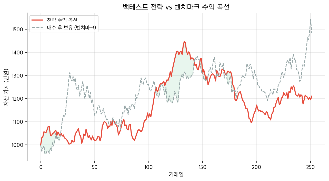
print(f"Average loss: {avg_loss:.3%}")

Step 5: Visualize the Results

Backtest strategy vs benchmark equity curve

import matplotlib.pyplot as plt

fig, (ax1, ax2) = plt.subplots(2, 1, figsize=(14, 8), sharex=True)

# Cumulative return comparison
ax1.plot(df.index, df['cumulative_market'], label='Market (Buy & Hold)')
ax1.plot(df.index, df['cumulative_strategy'], label='Strategy')
ax1.set_title('Cumulative Return Comparison')
ax1.legend()
ax1.grid(True, alpha=0.3)

# Drawdown
ax2.fill_between(df.index, drawdown, 0, alpha=0.3, color='red')
ax2.set_title('Strategy Drawdown')
ax2.set_ylabel('Drawdown (%)')
ax2.grid(True, alpha=0.3)

plt.tight_layout()
plt.savefig('backtest_result.png', dpi=150)
plt.show()

Key Pitfalls When Interpreting Backtest Results

Overfitting

If you iterate through parameter combinations (20-day, 60-day, etc.) to find the one with maximum profit, you likely have a strategy that only fits the past. If results change dramatically with a small tweak to the parameters, that is a warning sign.

No Look-Ahead Bias

Never assume you can trade at today’s closing price using today’s close. In reality you cannot know the closing price until after the close, so always assume entry at the next day’s open after a signal fires. Forgetting shift(1) introduces look-ahead bias.

Fees and Slippage

Excluding transaction costs inflates returns significantly. This effect is especially pronounced for high-frequency strategies.

Survivorship Bias

“Backtesting on Bitcoin gives great results” — that’s partly because Bitcoin survived. Running the same backtest on failed coins would give very different results.

Next Steps

This guide covers the most fundamental manual backtesting approach. To go further:

Use a backtesting framework: Backtrader, Vectorbt, Zipline
Walk-forward validation: Split data into training and test periods, then repeat iteratively
Multi-asset portfolio: Strategies across multiple instruments rather than a single asset
Risk management: Position sizing, stop-loss logic

Backtesting is not a tool for finding “a strategy that will make money” — it is a tool for confirming “this strategy does not work.” The real value is filtering out strategies that fail to pass.

Backtest Overfitting Prevention: Walk-forward vs Purged K-Fold Comparison

What to Look at Before IC When Combining Factors

What Is Quantitative Investing? A Beginner’s Guide for Individual Investors