Python Data Analysis Basics: Handling Stock Data with pandas

Why pandas?

Data analysis with pandas

Handling stock data requires working with numbers sorted by date. While Excel can do this, it becomes slow and difficult to automate when dealing with tens of thousands of rows.

pandas is the standard library in Python for working with tabular data. It’s widely used in quant analysis, data science, and financial modeling.

Installation and Getting Started

pip install pandas yfinance matplotlib

pandas: data analysis
yfinance: download free stock data from Yahoo Finance
matplotlib: plotting charts

Loading Stock Data

Bitcoin Data from Yahoo Finance

import yfinance as yf
import pandas as pd

# Bitcoin daily data (2 years)
btc = yf.download("BTC-USD", period="2y")
print(btc.head())

Sample output:

Open        High         Low       Close    Volume
Date
2024-04-08   69543.12   71842.15   68902.31   71015.94  32844900
2024-04-09   71015.94   71655.25   69241.84   69785.52  30492100
...

Column explanations:

Open: Opening price (first trade of the day)
High: Highest price during the day
Low: Lowest price during the day
Close: Closing price (last trade of the day)
Volume: Trading volume

Korean stock data

# Samsung Electronics
samsung = yf.download("005930.KS", period="1y")
print(samsung.tail())

Basic Data Exploration

Checking data size

print(f"Number of rows: {len(btc)}")
print(f"Period: {btc.index[0]} – {btc.index[-1]}")
print(f"Columns: {list(btc.columns)}")

Basic statistics

print(btc['Close'].describe())

This provides mean, min, max, standard deviation, etc.

Filtering specific periods

# Data only for 2025
btc_2025 = btc.loc['2025']

# First quarter of 2025
btc_q1 = btc.loc['2025-01':'2025-03']

Calculating Returns

Stock data and moving averages analyzed in pandas

A very common calculation in quant analysis.

Daily returns

btc['daily_return'] = btc['Close'].pct_change()
print(btc['daily_return'].tail())

pct_change() computes the percentage change from the previous day. For example, 0.03 indicates a 3% increase, -0.02 indicates a 2% decrease.

Cumulative return

btc['cumulative'] = (1 + btc['daily_return']).cumprod()
print(f"Total return: {btc['cumulative'].iloc[-1] - 1:.2%}")

Calculating Moving Averages

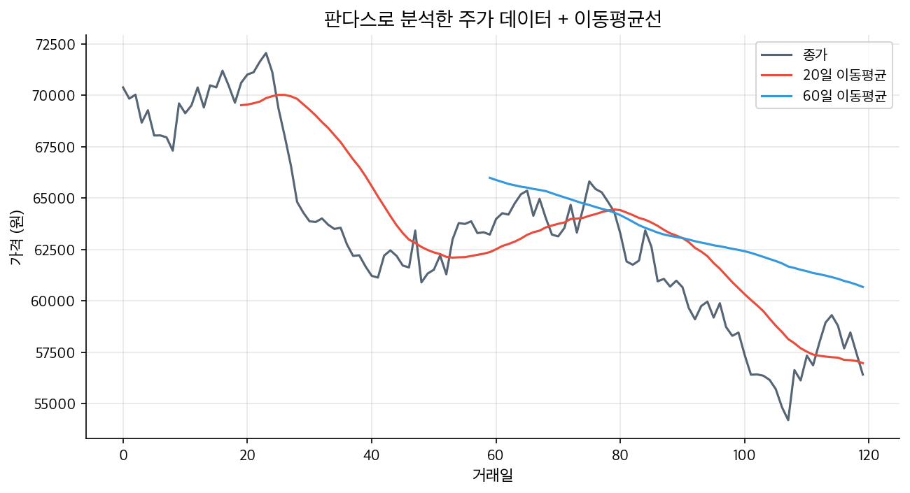
Moving averages smooth out price data by calculating the average over a set period. They are basic tools for identifying trends.

# 20-day moving average (short-term)
btc['ma20'] = btc['Close'].rolling(20).mean()

# 60-day moving average (mid-term)
btc['ma60'] = btc['Close'].rolling(60).mean()

# 200-day moving average (long-term)
btc['ma200'] = btc['Close'].rolling(200).mean()

Finding Golden Cross / Dead Cross

# Golden cross: short-term MA crosses above long-term MA
btc['golden_cross'] = (
(btc['ma20'] > btc['ma60']) &
(btc['ma20'].shift(1) <= btc['ma60'].shift(1))
)

golden_dates = btc[btc['golden_cross']].index
print(f"Number of golden cross events: {len(golden_dates)}")
for d in golden_dates[-5:]:
    print(f"  {d.date()}")

Plotting Charts

Close price + Moving Averages

import matplotlib.pyplot as plt

plt.figure(figsize=(14, 6))
plt.plot(btc.index, btc['Close'], label='Close Price', linewidth=1)
plt.plot(btc.index, btc['ma20'], label='20-day MA', linewidth=1)
plt.plot(btc.index, btc['ma60'], label='60-day MA', linewidth=1)
plt.title('Bitcoin Daily Chart')
plt.xlabel('Date')
plt.ylabel('Price (USD)')
plt.legend()
plt.grid(True, alpha=0.3)
plt.tight_layout()
plt.savefig('btc_chart.png', dpi=150)
plt.show()

Daily returns distribution

plt.figure(figsize=(10, 5))
btc['daily_return'].hist(bins=100, alpha=0.7)
plt.title('Bitcoin Daily Return Distribution')
plt.xlabel('Daily Return')
plt.ylabel('Frequency')
plt.axvline(0, color='red', linestyle='--')
plt.tight_layout()
plt.show()

Common pandas functions summary

Function	Example	Usage
Add column	`df['new'] = df['Close'] * 2`	Create new indicators
Filtering	`df[df['Close'] > 70000]`	Conditional selection
Sorting	`df.sort_values('Volume')`	Sort by volume
Grouping	`df.groupby(df.index.month).mean()`	Monthly averages
Handling missing data	`df.dropna()`	Remove NaNs
Saving	`df.to_csv('data.csv')`	Save to file

Next Steps

Working with pandas is the foundation of quant analysis. From here, three main directions are suggested:

Implementing Technical Indicators: Calculate and visualize RSI, MACD, Bollinger Bands, etc.

Backtesting: Develop trading rules and test their performance against historical data.

Automated Trading: Connect to exchange APIs for real-time trading automation.

No matter which path you choose, pandas will be a core tool. Mastering these basics will make advanced steps much easier.